Mahalanobis Distance

Many machine learning techniques make use of distance calculations as a measure of similarity between two points. For example, in k-means clustering, we assign data points to clusters by calculating and comparing the distances to each of the cluster centers. Similarly, Radial Basis Function (RBF) Networks, such as the RBF SVM, also make use of the distance between the input vector and stored prototypes to perform classification.

What happens, though, when the components have different variances, or there are correlations between components? In this post, I’ll be looking at why these data statistics are important, and describing the Mahalanobis distance, which takes these into account.

First, a note on terminology. “Covariance” and “correlation” are similar concepts; the correlation between two variables is equal to their covariance divided by their variances, as explained here. For our disucssion, they’re essentially interchangeable, and you’ll see me using both terms below.

Differences In Component Variances

Let’s start by looking at the effect of different variances, since this is the simplest to understand.

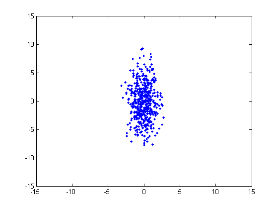
Consider the following cluster, which has a multivariate distribution. This cluster was generated from a normal distribution with a horizontal variance of 1 and a vertical variance of 10, and no covariance. In order to assign a point to this cluster, we know intuitively that the distance in the horizontal dimension should be given a different weight than the distance in the vertical direction.

We can account for the differences in variance by simply dividing the component differences by their variances.

First, here is the component-wise equation for the Euclidean distance (also called the “L2” distance) between two vectors, x and y:

Let’s modify this to account for the different variances. Using our above cluster example, we’re going to calculate the adjusted distance between a point ‘x’ and the center of this cluster ‘c’.

 

The Mahalanobis Distance

The equation above is equivalent to the Mahalanobis distance for a two dimensional vector with no covariance. The general equation for the Mahalanobis distance uses the full covariance matrix, which includes the covariances between the vector components.

Before looking at the Mahalanobis distance equation, it’s helpful to point out that the Euclidean distance can be re-written as a dot-product operation:

With that in mind, below is the general equation for the Mahalanobis distance between two vectors, x and y, where S is the covariance matrix.

(Side note: As you might expect, the probability density function for a multivariate Gaussian distribution uses the Mahalanobis distance instead of the Euclidean. See the equation here.)

The Mahalanobis Distance With Zero Covariance

Before we move on to looking at the role of correlated components, let’s first walk through how the Mahalanobis distance equation reduces to the simple two dimensional example from early in the post when there is no correlation.

Assuming no correlation, our covariance matrix is:

The inverse of a 2×2 matrix can be found using the following:

Applying this to get the inverse of the covariance matrix:

Now we can work through the Mahalanobis equation to see how we arrive at our earlier variance-normalized distance equation.

Correlation

So far we’ve just focused on the effect of variance on the distance calculation. But when happens when the components are correlated in some way?

Correlation is computed as part of the covariance matrix, S. For a dataset of m samples, where the ith sample is denoted as x^(i), the covariance matrix S is computed as:

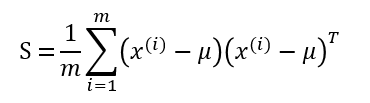
Note that the placement of the transpose operator creates a matrix here, not a single value.

For two dimensional data (as we’ve been working with so far), here are the equations for each individual cell of the 2×2 covariance matrix, so that you can get more of a feel for what each element represents.

If you subtract the means from the dataset ahead of time, then you can drop the “minus mu” terms from these equations.

Subtracting the means causes the dataset to be centered around (0, 0). It’s critical to appreciate the effect of this mean-subtraction on the signs of the values. Your original dataset could be all positive values, but after moving the mean to (0, 0), roughly half the component values should now be negative.

The top-left corner of the covariance matrix is just the variance–a measure of how much the data varies along the horizontal dimension. Similarly, the bottom-right corner is the variance in the vertical dimension.

The bottom-left and top-right corners are identical. These indicate the correlation between x_1 and x_2.

If the data is mainly in quadrants one and three, then all of the x_1 * x_2 products are going to be positive, so there’s a positive correlation between x_1 and x_2.

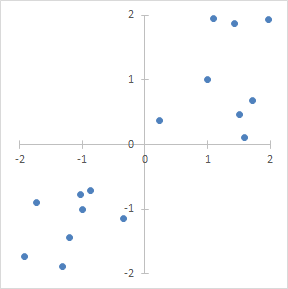
If the data is all in quadrants two and four, then the all of the products will be negative, so there’s a negative correlation between x_1 and x_2.

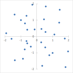
If the data is evenly dispersed in all four quadrants, then the positive and negative products will cancel out, and the covariance will be roughly zero. This indicates that there is no correlation.

As another example, imagine two pixels taken from different places in a black and white image. If the pixels tend to have the same value, then there is a positive correlation between them. If the pixels tend to have opposite brightnesses (e.g., when one is black the other is white, and vice versa), then there is a negative correlation between them. If the pixel values are entirely independent, then there is no correlation.

Effect of Correlation on Distance

To understand how correlation confuses the distance calculation, let’s look at the following two-dimensional example. The cluster of blue points exhibits positive correlation.

 

I’ve marked two points with X’s and the mean (0, 0) with a red circle. Looking at this plot, we know intuitively the red X is less likely to belong to the cluster than the green X. However, I selected these two points so that they are equidistant from the center (0, 0). Even taking the horizontal and vertical variance into account, these points are still nearly equidistant form the center.

It’s clear, then, that we need to take the correlation into account in our distance calculation.

The Mahalanobis distance takes correlation into account; the covariance matrix contains this information. However, it’s difficult to look at the Mahalanobis equation and gain an intuitive understanding as to how it actually does this.

We can gain some insight into it, though, by taking a different approach. Instead of accounting for the covariance using Mahalanobis, we’re going to transform the data to remove the correlation and variance.

We’ll remove the correlation using a technique called Principal Component Analysis (PCA). To perform PCA, you calculate the eigenvectors of the data’s covariance matrix. The two eigenvectors are the principal components. I’ve overlayed the eigenvectors on the plot. You can see that the first principal component, drawn in red, points in the direction of the highest variance in the data. The second principal component, drawn in black, points in the direction with the second highest variation.

Using these vectors, we can rotate the data so that the highest direction of variance is aligned with the x-axis, and the second direction is aligned with the y-axis. This rotation is done by projecting the data onto the two principal components.

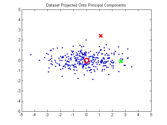
If we calculate the covariance matrix for this rotated data, we can see that the data now has zero covariance:

2.2396    0.0000

0.0000    0.3955

What does it mean that there’s no correlation? Just that the data is evenly distributed among the four quadrants around (0, 0). We’ve rotated the data such that the slope of the trend line is now zero.

You’ll notice, though, that we haven’t really accomplished anything yet in terms of normalizing the data. The two points are still equidistant from the mean. However, the principal directions of variation are now aligned with our axes, so we can normalize the data to have unit variance (we do this by dividing the components by the square root of their variance). This turns the data cluster into a sphere.

And now, finally, we see that our green point is closer to the mean than the red. Hurray!

Given that removing the correlation alone didn’t accomplish anything, here’s another way to interpret correlation: Correlation implies that there is some variance in the data which is not aligned with the axes. It’s still  variance that’s the issue, it’s just that we have to take into account the direction of the variance in order to normalize it properly.

The process I’ve just described for normalizing the dataset to remove covariance is referred to as “PCA Whitening”, and you can find a nice tutorial on it as part of Stanford’s Deep Learning tutorial here and here.

In this section, we’ve stepped away from the Mahalanobis distance and worked through PCA Whitening as a way of understanding how correlation needs to be taken into account for distances. Calculating the Mahalanobis distance between our two example points yields a different value than calculating the Euclidean distance between the PCA Whitened example points, so they are not strictly equivalent.